Lasso Regression

Before understanding Lasso Regression, let’s first understand Regularization.

What is Regularization?

Regularization means we regulate or constrain the model so that it does not overfit.

In simple words:

Regularization is a set of techniques used during model training to reduce overfitting by controlling model complexity.

When a model overfits, it performs very well on training data but performs poorly on unseen data. It becomes sensitive to small noise and the coefficients may become unstable or very large.

To solve this, we add a penalty term to the loss function.

There are three main regularization techniques:

1. Ridge Regression (L2 Regularization)

2. Lasso Regression (L1 Regularization)

3. Elastic Net (Combination of L1 and L2)

In this article, we will deeply understand Lasso Regression.

In Ridge Regression, we solved instability by shrinking coefficients.
But Ridge has one limitation:

It reduces weights, but it never makes them exactly zero.

That means even irrelevant features stay in the model.

So what if we want to reduce overfitting and automatically remove useless features. That is where Lasso Regression comes in.

Why Do We Need Lasso Regression?

Imagine you are working with 100 features out of which only 10 are actually important and 90 are noise.

In Ordinary Linear Regression, all 100 features get coefficients.
In Ridge Regression, all 100 features still get coefficients — just smaller ones.

However, when the size of problem grows, we often need a model that focuses only on relevant and important feature impacting the outcomes. This is called feature selection.

What is Lasso Regression?

Lasso Regression is a linear regression technique that adds an L1 regularization penalty to the loss function.

It is used to:

• Reduce overfitting

• Control model complexity

• Perform automatic feature selection

• Produce sparse models

Lasso stands for:

Least Absolute Shrinkage and Selection Operator

The key idea is that instead of minimizing only prediction error, we also penalize the absolute size of coefficients.

How Lasso Regression works?

In Linear Regression, we minimize Mean Squared Error (MSE):

$$Loss = \frac{1}{n} \sum_{i=1}^{n} (y_i - \hat{y}_i)^2$$

$$= \frac{1}{n} \sum_{i=1}^{n} (y_i - X\beta)^2$$

We already derived and studied the formula to calculate the B matrix which contains all the coefficients of the independent features. Its,

$$\begin{align} B &= (X^TX)^{-1}X^TY \end{align}$$

As we discussed with the example in Ridge regression, if features are highly correlated, if the number of features is large, or if data has noise, then the coefficients become unstable and large → high variance → overfitting(Derivation given in Ridge Regression (L2 Regularization)).

To control this, we add a penalty term. In lasso regression, the penalty term is:

$$L1 = | W | = |W_1| + |W_2| + |W_3| ... \text{and so on}$$

$$= \sum |\beta_j|$$

Let's say, if as the coefficients of features(β) increase due to the features being highly correlated, then the training error is small.

Without the penalty, the model says, "Good! Increase β more.”
With penalty, increasing β increases sum of absolute values of coefficients (Σ |β|) which increases total loss(as penalty term is directly added to loss function). So large β must justify its cost.

So, what Does “Justify Its Cost” Mean Mathematically?

Suppose we slightly increase one coefficient βj, then two things happen:

(A) MSE Changes - If the feature helps prediction, MSE decreases.

(B) Penalty increases - Because |βj| increased.

So the total loss change is:

$$ΔLoss=ΔMSE+λ⋅Δ∣βj∣$$

Now here is the KEY:

If increasing β reduces MSE by 0.5 but increases the penalty by 1. Then total loss increases.

So the model says:

Not worth it.

If increasing β reduces MSE by 5 and increases the penalty by 1. Then total loss decreases.

So the model says:

Worth it.

THAT is what “justify its cost” means.

Suppose a feature barely helps in predicting the target.

If you increase its coefficient slightly, then the MSE decreases only a tiny amount, but the penalty increases by λ× that increase.

If the penalty increase is larger than the error decrease, then the total loss increases, which means the model prefers to keep the coefficient at zero.

So mathematically, zero becomes the better choice.

The absolute value function |β| has a sharp corner at zero and because of that sharp corner, the optimization conditions allow zero to be an optimal solution even when the gradient from MSE is small.

In simple words:

If a feature’s effect on reducing error is smaller than λ,
then setting its coefficient to zero gives a smaller total loss.

So zero is not just allowed — it becomes optimal.

Overfitting happens when the model uses many small, noisy coefficients to slightly reduce training error.

Lasso reduces overfitting by saying, “A feature must reduce the error more than λ to stay in the model.” Thus, weak features cannot meet that requirement. So they are removed.

Why does lasso perform feature selection?

During optimization, the model searches for coefficient values that minimize this total loss.

For any feature βⱼ, two forces are acting at the same time:

1. The MSE term tries to adjust βⱼ in a way that reduces prediction error.

2. The L1 penalty tries to pull βⱼ toward zero.

Now here is the crucial difference between L1 and L2.

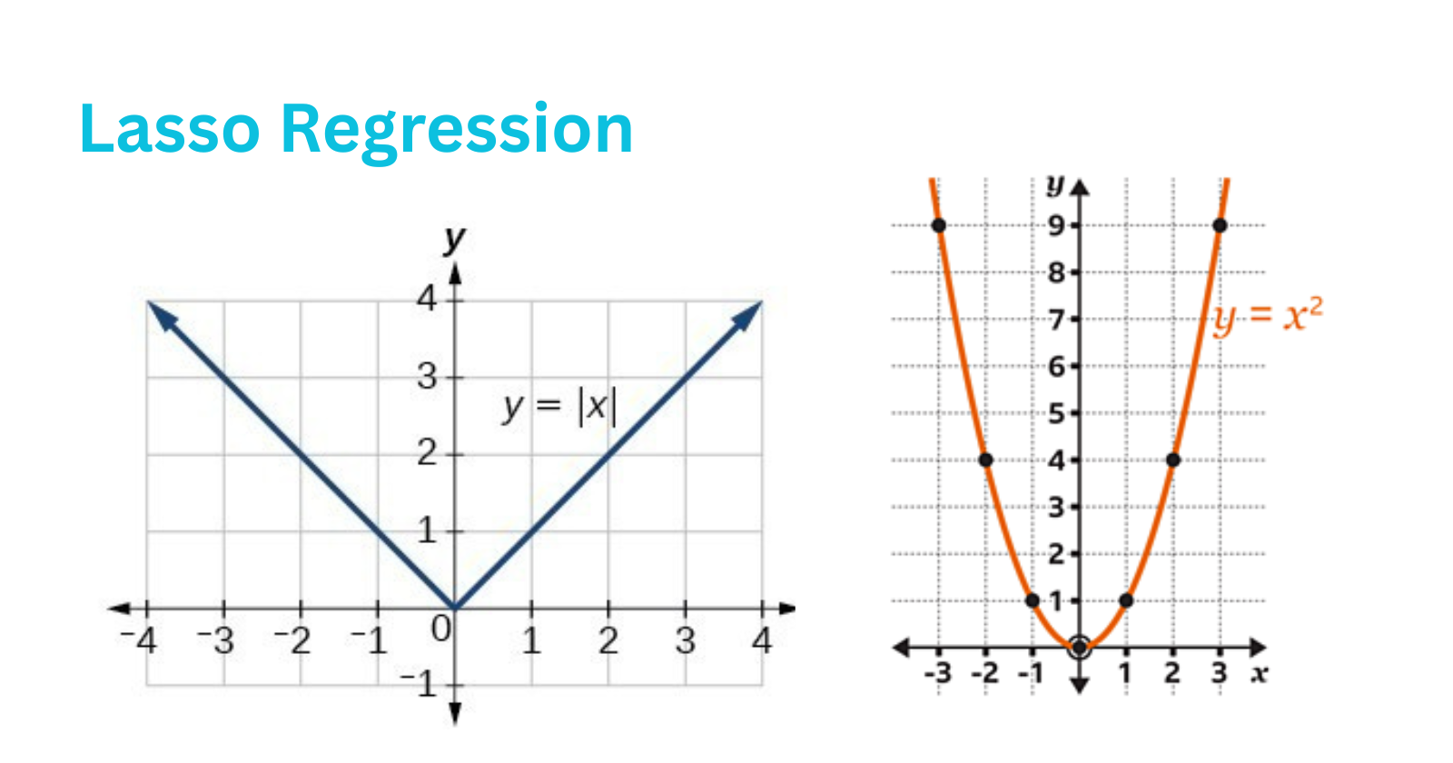
In Ridge (L2), the penalty term is β². Its derivative becomes smaller as β becomes small. That means near zero, the penalty effect is weak. So coefficients shrink, but they rarely become exactly zero.

In Lasso (L1), the penalty is |β|. The slope of |β| is constant (either +1 or -1) everywhere except at zero. This creates a sharp corner at zero.

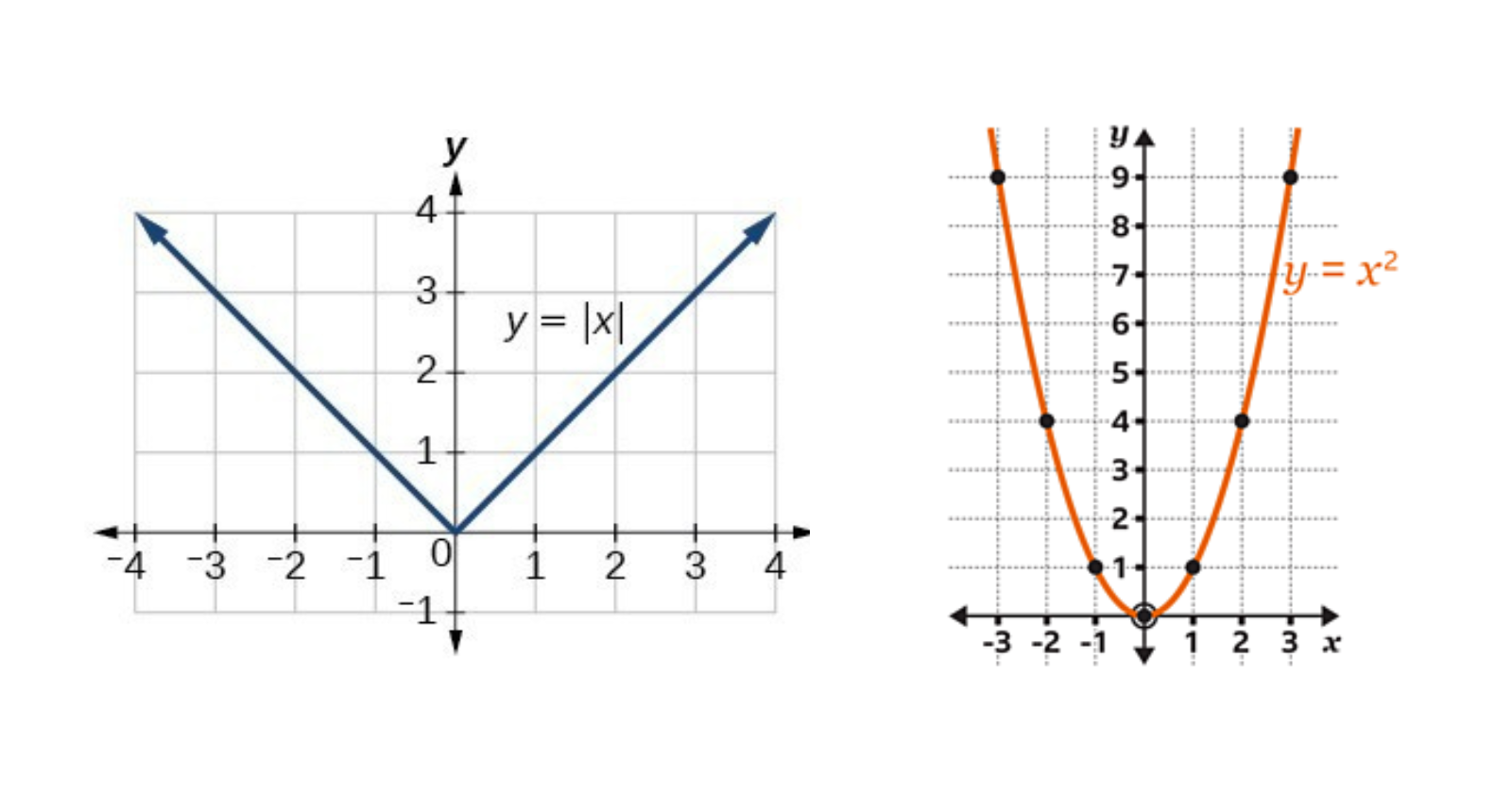
Because of this sharp corner, the optimization process allows zero to be a stable minimum.

This means:

If a feature contributes only slightly to reducing the MSE, the constant pull from the L1 penalty dominates and pushes the coefficient exactly to zero.

That is why Lasso performs feature selection.

Advantages of Lasso Regression

1. Automatic Feature Selection
   Lasso can set some coefficients exactly to zero, removing irrelevant features from the model.

2. Reduces Overfitting
   Eliminating weak predictors, it reduces variance and improves generalization.

3. Produces Sparse Models
   Sparse models are easier to interpret and computationally efficient.

4. Useful for High-Dimensional Data
   Especially effective when the number of features is large (e.g., text data, genomics).

Disadvantages of Lasso Regression

1. Struggles with Highly Correlated Features
   If two features are strongly correlated, Lasso may randomly choose one and discard the other, even if both are important.

2. Can Underfit if λ is Too Large
   A very large penalty can remove important features.

3. No Closed-Form Solution
   Unlike Ridge, Lasso does not have a simple matrix inverse solution and requires iterative optimization methods.

4. Biased Coefficient Estimates
   Because coefficients are shrunk, estimates are biased compared to ordinary least squares.

Conclusion

Lasso Regression works by adding an L1 penalty to the loss function, which introduces a fixed cost for every non-zero coefficient.

A feature must reduce prediction error more than this cost to remain in the model. If it does not, the optimal solution for its coefficient becomes exactly zero.

Because of the sharp corner of the absolute value function at zero, Lasso naturally produces sparse solutions, automatically performing feature selection.

By removing weak and noisy features, Lasso reduces model complexity, lowers variance, and improves generalization on unseen data.