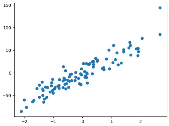
We have covered simple and multiple linear regression so far. Both of them deal with data that is linear as given in the figure below.

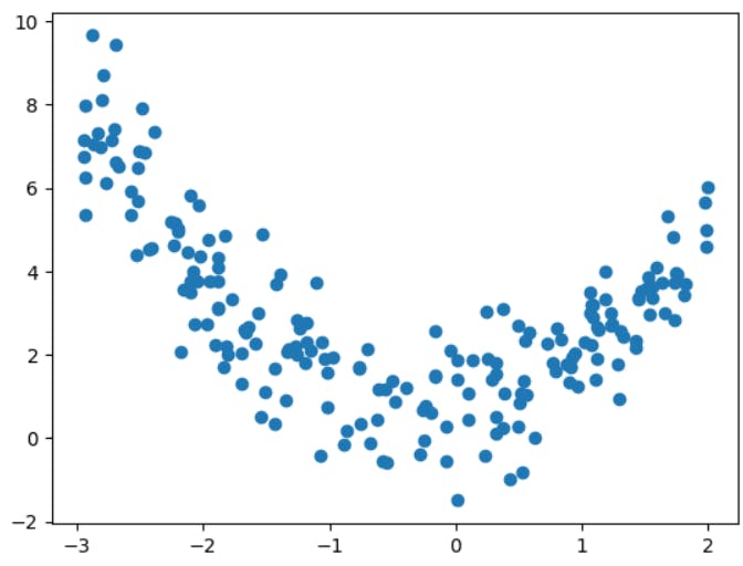
But as you work on real world problems, you will not obviously have a linear data everytime. Therefore, your data may look like this.

Or this!

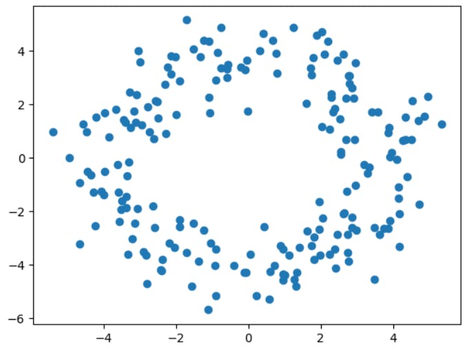
In either of these scenarios, linear regression would fail to perform better as the relationship is not linear and the error would be high. Therefore, we must use polynomial regression in such a case.

What is Polynomial Regression?

Let's first understand the word "polynomial". Polynomials are sums of terms of the form k⋅xⁿ, where k is any number and n is a positive integer. For example, 3x² + 7x+ c =0 is a polynomial.

Thus, polynomial equations help us define the figures that are not linear, they could be parabolic, circular, etc. You might have studied in mathematics that the equation of parabola and circle is given by y²\= 4ax and x²+y²\= a respectively. Both are polynomial equations having a degree of 2.

Now that you know what a polynomial equation is, you might have guessed what we are about to do next. Smart you!

We must fit this equation to the given data to capture the relationship. I'll show you exactly how, but before that let's take a look at the definition of Polynomial Regression.

Polynomial Regression is a type of regression algorithm in which the relationship between the independent variable x and the dependent variable y is expressed as an nth degree polynomial in x.

Using Polynomial Regression

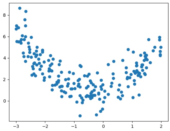
Let's say you have the following data represented on the scatter plot.

CASE 1: USE LINEAR REGRESSION

Now just for fun, let's see how it looks if we apply linear regression on it.

from sklearn.model_selection import train_test_split
from sklearn.linear_model import LinearRegression
from sklearn.metrics import r2_score
from sklearn.datasets import make_regression
import pandas as pd
import numpy as np

X = 5 * np.random.rand(200, 1) - 3
y = 0.85 * X**2 + 0.7 * X + 1 + np.random.randn(200, 1)

X_train,X_test,y_train,y_test = train_test_split(X,y,test_size=0.2,random_state=2)
lr = LinearRegression()
lr.fit(X_train,y_train)
LinearRegression()
y_pred = lr.predict(X_test)
print(r2_score(y_test,y_pred))

If you run the above code, you will see that the r2 score is around 0.017060049924691456 which is worse and clearly explains that model is not performing well on data. (You might get a slightly different value since the random function will be generating different random numbers everytime you run the code).

In fact, you can see the line that it has fitted on the data below.

plt.plot(X_train,lr.predict(X_train),color='r')
plt.plot(X, y, "b.")
plt.xlabel("X")
plt.ylabel("y")
plt.show()

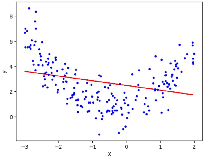
Now you know how bad the situation is!!😬

CASE 2: USE POLYNOMIAL REGRESSION

Clearly, we see why we must not use linear regression for such datasets. Therefore, let's explore the PolynomialFeatures class offered by scikit learn.

from sklearn.preprocessing import PolynomialFeatures,StandardScaler
poly = PolynomialFeatures(degree=2,include_bias=True)

X_train_trans = poly.fit_transform(X_train)
X_test_trans = poly.transform(X_test)

Here, we have specified degree as 2 and bias as 'True' as arguments for PolynomialFeatures. This will give us feature x raised to the power 2, 1 and 0. You can check this by using .powers_ method as given below.

poly.powers_

Output: array([[0], [1], [2]])

Therefore, before using this particular class, your data had only one independent variable, i.e. x. After using PolynomialFeatures, you have x² , x and x⁰ (means 1, i.e. bias term) as in three features. Now, these three features can be used to calculate our dependent variable y. Note that you can set the include_bias=False to get only two features and no bias term (such as only x² and x). However, most of the time we keep it True.

So, now that you have three features ready, we are ready to find out the relationship between these three to get our y value. It means, we must find values of b0, b1 and b3 in the equation given below since we already have the terms of x raised to power 0, 1 and 2.

$$y = \beta_2 x^2 + \beta_1 x + \beta_0 c + d$$

To achieve this, we use linear regression class, as given below,

lr = LinearRegression()
lr.fit(X_train_trans,y_train)
y_pred = lr.predict(X_test_trans)
r2_score(y_test,y_pred)
print(lr.coef_)
print(lr.intercept_)

The three coefficients(betas) and intercepts(d term) are [0, 0.80182357, 0.89323134] and 0.93858425 respectively.

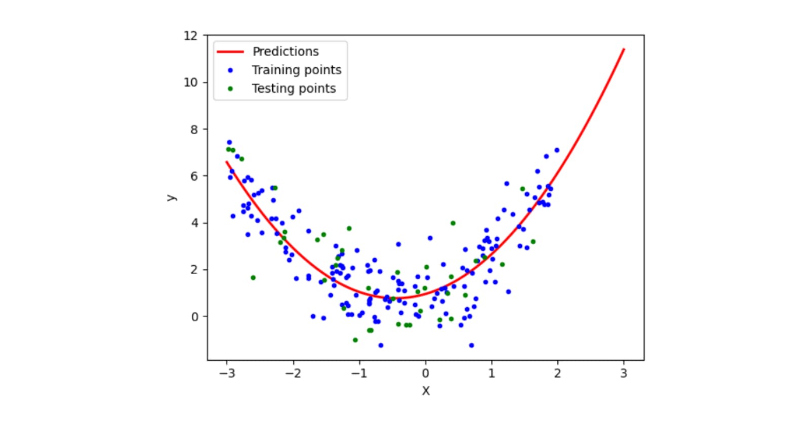
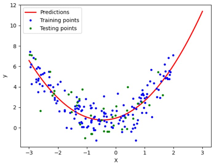
Let's plot it and see how the line fits now.

X_new=np.linspace(-3, 3, 200).reshape(200, 1)
X_new_poly = poly.transform(X_new)
y_new = lr.predict(X_new_poly)

plt.plot(X_new, y_new, "r-", linewidth=2, label="Predictions")
plt.plot(X_train, y_train, "b.",label='Training points')
plt.plot(X_test, y_test, "g.",label='Testing points')
plt.xlabel("X")
plt.ylabel("y")
plt.legend()
plt.show()

print(r2_score(y_test,y_pred))

When you check the R2 score, it will be around 0.8 which shows that the model has improved a lot since we used polynomial features instead of directly applying linear regression.

Well, if you are a math geek and wondering where is the fun math part in this article then sorry to disappoint you. The equations that I mentioned above were the only maths part here.😂

And if you hate math, lucky you! I bet this was the easiest one for you that you would remember in the long run.

Conclusion

Trust me! You are doing awesome! We have covered three regression algorithms so far and there are still a lot more algorithms to go. But don't you worry, they are super easy and I hope I'm able to deliver it well to you.

Also, don't think much that you are still stuck on the regression algorithms so far because, to be honest, they are the first and most important stepping stones. Once we finish all the regression algorithms we will move towards classification algorithms. And that way you would have covered all the algorithms in Supervised Machine Learning. Things are right around the corner, don't rush! Take your time and let the knowledge sink in. See you in the next article!